Quantitative Mass Spectrometry with spectro_inlets_quantification
Author: Spectro Inlets
Date: November 2020
Introduction: A new window through which to count molecules
A clear goal of mass spectrometry, with value in countless chemical and biochemical applications, is to determine the composition of a medium. This can mean:
A. The concentration of volatile components in a liquid or, similarly,
B. The partial pressure of components of a gas.
A related goal, with value in more niche applications such as catalysis and electrocatalysis research, is to determine:
C. The absolute number of a particular molecule produced in a given time (its flux).
The term quantification can refer to determination of either of the three quantities above.
Mass spectrometry in principle makes this possible by registering a signal at a unique subset of m/z values in response to a given analyte molecule in the liquid or gas. The physics behind this, separated into seven transfer steps from dissolved analyte to raw signal from the detector, is described in Section Step-by-step physics of MS of this Application Note and motivates our approach to quantitative mass spectrometry. Despite each of these steps being researched and described in academic literature and/or the documentation of established commercial providers of mass spectrometer solutions, a robust, versatile, and stable on-line quantification method based on mass spectrometry has been elusive.
Spectro Inlets approaches this problem informed by two unique advantages:
Spectro Inlets’ core chip-based vacuum inlet technology. This is a very well-defined and highly reproducible inlet. We know the exact dimensions of the chip capillary, and can quantitatively predict the rate at which it lets molecules into the mass spectrometer.
Spectro Inlets’ experience in Electrochemistry - mass spectrometry (EC-MS). EC-MS enables experiments in which the absolute molecular flux with which a given molecule is entering the mass spectrometer (denoted \(\dot{n}^i\)) is directly under control. This experiment, called internal calibration and briefly described in Section Determining sensitivity factors, gives us a direct probe of the absolute sensitivity factor (denoted \(F^i_M\)). This enables verification of the capillary flux.
Though these two advantages only give direct new insight into vacuum inlet, one of seven transfer functions between a dissolved analyte and a mass spec signal, it proves to be the missing piece that can bring quantitative mass spectrometry to a practical reality. Sections Quantification strategy and Determining sensitivity factors below describe how this approach gives both practical advantages and theoretical insight. In short, it involves treating the absolute flux of molecules through the vacuum inlet as a fundamental quantity which is the key also to quantification of an analyte in a bulk liquid or gas.
Sections Overview of the modules of spectro_inlets_quantification describe the code package, spectro_inlets_quantification, developed in python to represent the physics and implement the quantification strategy described in Sections Step-by-step physics of MS - Determining sensitivity factors. This Application Note serves as a general documentation of spectro_inlets_quantification v1.0 so code examples are provided in the text of sections Overview of the modules of spectro_inlets_quantification. An accompanying Ipython notebook to this document contains code examples which make all of the included figures (unless otherwise noted) and demonstrate the modules of spectro_inlets_quantification. On the other hand, this Application Note falls short of prescribing experimental procedures, which is application-specific and should be developed by the user and/or documented elsewhere.
Step-by-step physics of MS
This section goes through all the steps from a molecule dissolved in a liquid to an ionized fragment of that same molecule hitting the detector of the mass spectrometer and causing a signal to be recorded or show up on our screen.
It has to (1) evaporate, (2) enter the vacuum chamber, (3) get to the ionization chamber, (4) get ionized (5) fragment (or stay together), (6) make it through the mass filter, and (7) create a signal at the detector.
This may be an exciting and unpredictable journey for an individual molecule, with the success and the timing of each of the above steps a matter of chance. However, even at the lowest detectable concentration (or partial pressure or flux) of analyte, millions of molecules are making this journey every second, so from our point of view the law of large numbers takes all the surprise out of it. We further rob individual molecules of any remaining agency by operating under the assumption of linearity. That means that, all else equal, for a given increase in the concentration of analyte, there’s a proportional increase in the signal.
The assumption that the signal responds linearly to amount, all else equal, depends on the transfer functions of each of the seven steps above being constant with respect to the amount of our particular molecule, at least over some concentration range. Figure 1 shows an overview of the steps and their transfer functions, and the intermediate quantities whose proportionality is given by that transfer function.
The next subsections describe each step, the transfer function, its dependencies, and the assumptions that support it or could further strengthen it.
This Application Note focuses on the case where the analyte starts dissolved in a liquid (case A above), as this involves all seven transport steps. The quantification problem becomes simpler if you are only interested in quantification of the flux (C above) and/or partial pressure (B) of analyte molecules, rather than the concentration. In that case, consideration of the evaporation and/or capillary flux steps described below may not be necessary.
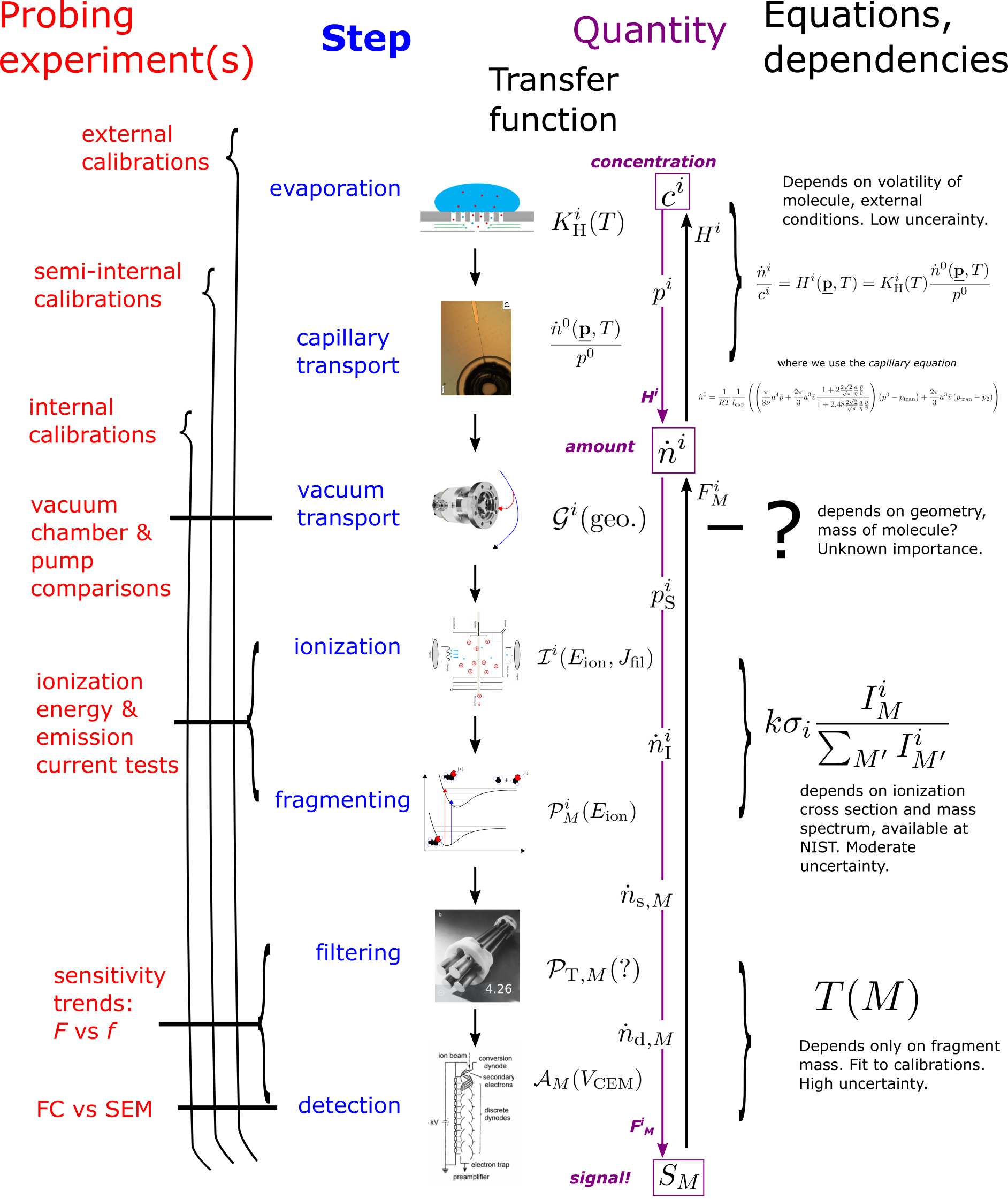
Fig. 1 Overview of Quantification by MS. The figure for step 4 is from wikipedia and the figures for steps 6 and 7 are from the Mass Spectrometry textbook.
Note on Notation
We introduce a symbol for each transfer function and intermediate quantity. In the following sections we will reduce the problem, to minimize the number of quantities we actually have to work with in practice.
The analyte molecule throughout this Application Note is called \(i\), and variables that depend on molecule type will have a superscript \(^i\). The m/z ratio at which we are measuring the signal is called \(M\), and all variables that depend on the state of the mass spectrometer (most importantly the mass-filtering voltages that control m/z) during detection will have a subscript \(_M\). The superscript \(^0\) indicates total over molecules, i.e. \(\sum^i\). Other known dependencies are, to the degree possible, indicated with parentheses after the transfer function.
Evaporation
In evaporation, the molecule leaves the liquid \(i\), where it has concentration \(c^i\), and enters the gas (in the chip sampling volume), where it has partial pressure \(p^i\). The transfer function is the ratio of \(p^i\) to \(c^i\). This transfer function is, by definition, the Henry’s-Law constant \(K_\text{H}^i\):
Dependencies
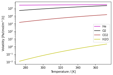
Fig. 2 Volatility constants of a few common molecules dissolved in water as a function of temperature from 0 to 100 \(^\circ\) C. The volatility constant of water is its vapour pressure divided by the molar concentration of pure water (55,500 [mol/m^3]).
The Henry’s law volatility constant is a function of temperature (\(T\)) according to
where \(K_\text{H,0}^i\) is the volatility constant at the standard temperature of \(T_0=\)298.15 [K] (25 \(^\circ\) [C]) and \(T_c^i\) is the temperature dependence constant for analyte \(i\). The Henry’s-Law solubility constants \(H_0^i = 1/K_\text{H,0}^i\) and temperature dependence constants \(T_c^i\) are tabulated for a huge collection of molecules in Sanders’ compilation available at http://doi.org/10.5194/acp-15-4399-2015.
The volatility constants of a few common molecules are shown as a function of temperature in Figure 2.1
Assumptions
The transfer function in Equation (1) is subject to the following assumptions:
Assumption 1
The concentration of analyte \(i\) is equal to the concentration of analyte at the membrane, i.e. \(c^i(y\!=\!0) = c^i\).
This is the assumption that the analysis liquid is well-mixed. This implies that we are not depleting \(i\) at the membrane.
Assumption 2
The Henry’s Law constant does not depend on the concentration of analyte \(i\).
This assumption is required for linearity. It is only expected to hold for rather dilute solutions, as Henry’s-Law is defined as the limiting volatility as \(c\rightarrow 0\). It is a sub-assumption of this more general assumption:
Assumption 3
The Henry’s Law constant does not depend on the composition of the liquid.
This is likewise only valid for dilute aqueous solutions. With a very different solution, such as a nonaqueous solvent, it’s necessary to find and use a Henry’s-Law constant specific to that solvent.
Assumption 4
The Henry’s Law constant does not depend on the pressure or composition of the gas.
This assumption will usually hold well because at \(T\ge 298\) K and \(p<10\) bar, most gases behave ideally.
Capillary transport
During measurement, the sampling volume of the chip is constantly leaking into the vacuum chamber via the chip capillary. The transfer function is the ratio of the flux of \(i\) through the capillary, \(\dot{n}^i\), to its partial pressure in the chip, \(p^i\). We will assume, as described below, that the capillary is taking a representative sample of the sampling volume. This transfer function, then, with the assumptions below, is the total capillary flux \(\dot{n}^0\) divided by the total pressure in the chip \(p^0\).
Dependencies
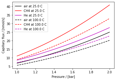
Fig. 3 Flux of air, CH\(_4\), and He through the chip at two temperatures as a function of pressure according to Equation (4)
The transfer function depends on total chip pressure \(p^0\) and the total capillary flux, \(\dot{n}^0\).
\(p^0\) must be measured. If the chip is open to air, it will be approximately 1 [bar] or 10\(^5\) [Pa].
The capillary flux, \(\dot{n}^0(\underline{\mathbf{p}}, T)\), is calculated from a number of properties of the gas flowing through the capillary as follows:
The flow of molecules through the capillary goes through at least three regimes as the pressure drops from 1 bar to high vacuum [Henriksen2009]: (1) a viscous flow regime near ambient pressure, (2) a transition regime, and (3) a molecular flow regime governed by Kundsen diffusion near high vacuum. It is therefore not trivial to derive an analytical expression, but this has been done. The capillary equation is [Trimarco2017, Equation 4.10]:
Here, \(p^0\) is the inlet pressure, \(p_2\) is the outlet pressure (\(\approx\) 0), \(p_{\mathrm{tran}}=\frac{k_B T}{2 \sqrt{2}\pi s^2 a}\) is the pressure at which the transition from viscous to molecular flow occurs, \(\bar{p}=\frac{p^0 + \bar{p}_{\mathrm{tran}}}{2}\) is the average pressure in the viscous flow regime, \(\eta\) is the viscosity of the gas, \(s\) is the molecular diameter, \(\bar{v}=\sqrt{\frac{8 k_B T}{\pi m}}\) is the mean thermal velocity of the gas molecules, and \(m\) is the molecular mass. Furthermore, \(l_\text{cap}\) is the length of the capillary, and \(a=h_\text{cap}=w_\text{cap}\) is its height and width, assumed to be equal (square cross-section). By design, \(l_\text{cap} = 1\,\text{mm}\), \(w_\text{cap} = 6\,\mu\text{m}\), and \(h_\text{cap} = 6\,\mu\text{m}\). This equation is plotted for a few common gases in Figure 3.
The capillary equation thus depends on the viscosity \(\eta\), molecular diameter \(s\), and molecular mass \(m\) of the gas in the sampling volume. These can be looked up for a pure gas.
But what if the gas in the sampling volume is a mixture?
For the viscosity, we rely on the viscosity of mixtures calculation in Davidson1993, which takes the molecular masses, viscosities, and mol fractions of the components and applies the kinetic theory of gases. An example (O\(_2\) in He) is shown in Figure 4.
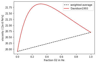
Fig. 4 Viscosity of a He-O\(_2\) calculated by weighted average (black dotted) and by the method in Davidson1993 (red solid). The increased viscosity has to do with the inefficient transfer of momentum between the smaller He and larger O\(_2\)
For molecular diameter and molecular mass, we rely (for now) simply on a weighted average. Since the mol fraction of a component is proportional to its partial pressure, we can write this for a property \(X\) as
The capillary flux equation also depends on the capillary geometry. It assumes that the depth=width=\(a\) and the length=\(l_\text{cap}\).
With EC-MS, it is possible to verify the capillary equation. As seen in Figure 1 and described in more detail in Section Determining sensitivity factors, the capillary flux can be isolated by comparing internal and semi-internal calibrations.
The easiest way to do this in practice is to compare the signal at m/z=32 for O\(_2\) made by electrochemical oxygen evolution (known \(\dot{n}^i\)) and for O\(_2\) in air (known \(p^i\)), and then equate the two by replacing \(l_\text{cap}\) with \(l_\text{eff}\). In reality, it is the depth that varies and not the length, but it is easier to solve for an effective capillary length \(l_\text{eff}\), since the total flux is proportional to one over the capillary length (Equation (4)).
\(l_\text{eff}\) is typically within \(\pm\)3% of the actual \(l_\text{cap}=1\)mm.
Assumptions
The transfer function in Equation (3) is subject to the following assumptions:
Assumption 5
The partial pressure at the capillary inlet is equal to the partial pressure at the membrane, i.e. \(p^i=p^i(y\!=\!0)\), i.e., the gas is well-mixed.
This assumption is analogous to Assumption 1. This assumption has high confidence, since gas diffusion is very rapid at the length scales of the chip sampling volume size.
Assumption 6
The rate at which molecules go through the capillary is proportional to their partial pressures at the capillary entrance. In other words, the capillary has no separation effect.
This assumption is reasonable because start of the capillary is in viscous flow regime, where the whole gas moves together as a continuum fluid, so there is no separation effect due to the capillary. Maybe there are separation effects later, when the pressure drops to the molecular flow regime, but these separation effects have no way of communicating back up through the viscous flow regime to the bulk. So they can’t have an effect on the rate at which gas is entering the capillary. They can, in principle, cause a small build-up of one compound relative to another in the middle of the capillary, but at steady state (aka dynamic equilibrium), the rate at which molecules are entering has to be the rate at which molecules are exiting the capillary.
Assumption 7
The capillary is the only way for gas to get out of the sampling volume.
… in other words, that there is no back diffusion through the carrier gas delivery channels. This assumption is needed for internal calibration, described in Section Determining sensitivity factors.
The critical and new assumption, an assumption that we can verify, is that we know \(\dot{n}^0\):
Assumption 8
The total flux through the capillary obeys the capillary equation.
The capillary equation is Equation (4) above.
Finally, to use it for a mixed gas, we assume the following about the gas in the capillary:
Assumption 9
A transport property of a mixed gas is the mol-weighted average of that transport property for its components, with the exception of viscosity. The viscosity of a mixture can be calculated by the method in Davidson1993.
Vacuum transport
When a molecule has made it through the capillary into the vacuum, it has to get to the ionization source and stay there long enough to be ionized, rather than finding its way to the pump first. The transfer function to describe this is the ratio of the partial pressure of \(i\) in the ionization source \(p_\text{S}^i\) to the rate at which \(i\) is coming through the capillary, \(\dot{n}^i\). Because this ratio depends mostly on the geometry of the setup, defined to include the pump size and location, we’ll use \mathcal{G} = \(\mathcal{G}\) for it.
Dependencies
In principle, \(\mathcal{G}^i\) may depend on properties of the molecule \(i\), for example its stickiness to the vacuum walls and its molecular mass.
However, our experiments indicate that \(\mathcal{G}\) does not depend on the identity of the molecule, so long as the roughing pump prevents back diffusion. This is the case for a scroll pump with 1 bar gas in the chip.
Assumptions
We assume the following, valid to our knowledge with the use of a powerful roughing pump:
Assumption 10
The vacuum transport transfer function is a constant.
Or, as an equation:
Ionization
When a molecule is in the ionization source, it can get hit by an electron originating from the filament, giving it enough energy to knock one of its own electrons loose. The transfer function is the ratio of the rate at which \(i\) is ionized, \(\dot{n}_\text{I}^i\), to its partial pressure at the ion source, \(p_\text{S}^i\). We’ll call this \(\mathcal{I}\).
Dependencies
The ionization transfer function, as indicated in Equation (7), depends on the state of the ionization source. In electron impact ionization, that includes the voltage that the ionizing electrons are accelerated through, the ionization energy (\(E_\text{ion}\)); and the rate at which ionizing electrons are emitted, the filament current (\(J_\text{emis}\)). It also depends on how easy it is to ionize the molecule - this is described by a parameter called the ionization cross-section, denoted \(\sigma\). This cross-section is a function only of the ionization energy.
Assumptions
The ionization cross-section is used in the following assumption:
Assumption 11
For a given emission current and ionization energy, the rate at which molecule \(i\) is ionized is proportional to its ionization cross section \(\sigma^i= \sigma ^i(E_\text{ion})\):
As an equation, this is
These ionization cross-sections are generally available in the literature (for example NIST chemistry webbook). They can be measured by calibrating an ion gauge against a pressure sensor based on another mechanism.
The linearity and ideality assumption plays a role here:
Assumption 12
A molecule’s chances of being ionized don’t depend on how many of that or other molecules there are, i.e., \(\mathcal{I}^i(E_\text{ion}, J_\text{emis})\) does not depend on \(\underline{p}_\text{S}\)
Fragmenting
The transfer function for fragmentation is the rate at which fragments of mass \(M\) are generated in the ion source (\(\dot{n}_{\text{s}, M}\)) to the total rate at which the parent molecule \(i\) is ionized (\(\dot{n}_{\text{I}}^i\)). It is dimensionless and can be considered a probability, so we’ll use \mathcal{P} = \(\mathcal{P}\) for it, with both \(i\) and \(M\) dependencies:
Dependencies
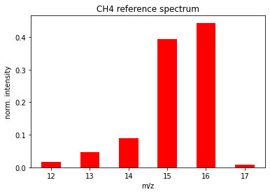
Fig. 5 Normalized CH\(_4\) spectrum (cracking pattern) from the NIST webbook for CH\(_4\).
The probability that an ionization event will result in a fragment with m/z=\(M\) is very difficult to produce but straight-forward to measure. It is approximately the portion of the mass spectrum of \(i\) that is peak \(M\). If \(I_M^i\) is the (relative) intensity at \(M\) in the mass spectrum of \(i\), then
For this to be useful a priori, trusted reference spectra need to be available. A free and very convenient library of reference spectra exist on the NIST webbook at https://webbook.nist.gov/. Figure 5 shows \(\mathcal{P}^{{{CH4}}}_M\) according to the NIST reference spectrum for CH\(_4\).
However, in our experience the reference spectra there are in general incomplete and/or somewhat inaccurate for most molecules as measured by quadrupole mass spectrometry in-house (See the Ipython notebook under the calibration module). The NIST reference spectra, furthermore, do not specify the ionization energy.
Double-ionization is a different process than fragmentation. Double-ionization is predominantly the result of two electron impact events, whereas fragmentation is the result of excess energy from a single electron impact event. Thus, double ionization depends on \(J_\text{emis}\) whereas fragmentation only depends on \(E_\text{ion}\). Double ions will also have a very different detector amplification (step 7), and so should be avoided. An easily double-ionized species, Ar, should have, according to NIST, a double ion signal portion of about 10% (this is the case for our in-house calibrations, see the Ipython notebook), and thus presumably an even smaller flux portion.
Assumptions
We also assume linearity and ideality in fragmentation:
Assumption 13
The fragmentation pattern of an ion does not depend on how many of that or other ions there are.
Also, because doubly-charged fragments would behave differently than the much more common singly-charged fragments, we wish to ignore their contribution. Some molecules have a high tendency to double-ionize, such as Ar, but most other molecules have much less than 10% double-ionized fragments. We assume:
Assumption 14
The mass of ions can be assumed proportional to the m/z ratio. I.e., z will be assumed to be 1.
Filtering
Everything from the generation of the charged fragment at m/z=\(M\) to its impacting the detector, we’ll group as “filtering”. The most important part of filtering is the quadrupole, which is typically operated to only “transmit” (or let through) fragments of a specific mass-to-charge ratio.
The transfer function is the ratio of the rate at which ions at \(M\) are hitting the detector, \(\dot{n}_{\text{d}, M}\), to the rate at which they are generated in the ion source, \(\dot{n}_{\text{s}, M}\). It is also a dimensionless probability, which we will call \(\mathcal{P}_\text{T}\) where the T stands for transmission.
Dependencies
Ideally, the probability of an ion with m/z=\(M\) being transmitted through the quadrupole filter, when the quadrupole is set to filter for m/z=\(M\), should be high and constant. In reality, it is not constant due in part to fringe effects right before and after the start of the quadrupole (Joseph2018) which effect higher masses more strongly, and in part to the fact that a narrower relative resolution is required to keep a constant m/z resolution as the m/z number increases (Douglas2009). Both of these imply it should be a function of \(M\). As a working approximation, we guess that it is a constant times a power of the m/z number \(M\):
We will consider this a hypothesis rather than an assumption, and test it later on.
Assumptions
We again assume linearity and ideality.
Assumption 15
The probability of an ion with m/z=\(M\) making it through the quadrupole does not depend on how many of that ion or other ions there are.
Detection
Finally, the ion fragments hit the detector, resulting in a measurable current, which is the signal.
This transfer function is actually an amplification function, the ratio of the signal generated \(S_M\) to the rate at which ions of m/z=\(M\) are hitting the detector, \(\dot{n}_{\text{d}, M}\). It gets a \mathcal{A} = \(\mathcal{A}\)
Dependencies
For a Faraday Cup, the ‘‘amplication function’’ is in theory just Faraday’s constant:
For a channel electron multiplier, the amplification factor is some much larger number that depends on the CEM voltage. It also depends on the mass of the fragment impacting the CEM. One source(Joseph2018) says that the number of electrons ejected on the first impact (so far the same for CEM and SEM) is proportional to the inverse square root of the mass of the ion.
Assumptions
The only assumption to make here a priori is that of linearity, i.e.
Assumption 16
The signal per ion impacting the detector at m/z=\(M\) making it through the quadrupole does not depend on how many of that ion are hitting the detector.
Quantification strategy
This section applies the physics described above to suggest a strategy for quantifying signals, i.e. calculating a set of concentrations, \(\vec{c}\), from a set of signals, \(\vec{S}\). The key is to make a distinction between the “external steps” to and including the vacuum inlet (Subsection The mass transfer coefficient H in [m^3/s]) and the “internal steps” that take place in the vacuum chamber (Subsections The absolute sensitivity factor F in [C/mol] and Predicting sensitivity factors (F-vs-f)).
First, though, we have to be a bit more precise what we mean by a “signal”.
Defining the signal
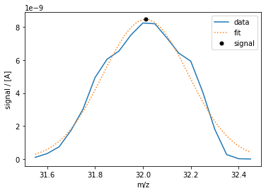
Fig. 6 M32-CEM peak and signal using a Gauss fit.
The word signal in its broadest term just refers to the output of the mass spectrometer, i.e. raw data. However in \text{quant.physics} it takes on another meaning as well:
Definition 1
A signal \(S_M\) is a single number in [A] resulting from a well-defined measurement by a mass spectrometer, where the subscript \(M\) defines the measurement. Typically the signal is the height of the peak around an integer m/z ratio at a given mass spec setting, so \(M\) is the combination of the m/z value and the setting.
This can often be approximated sufficiently as the read-out of the mass spectrometer set to the desired m/z, as data is acquired in Multiple Ion Detection (MID) mode, in which case the raw data is the signal.
A disadvantage to this simple MID is that it is sensitive to changes over time in peak center or shape. A more robust way to define the signal is advanced MID, whereby a scan is made around a peak and its height is fitted. An example of this for the peak centered around m/z=32 as measured with a CEM detector with air in the chip is shown in Figure 6. The signal is the height of the gauss curve which fits the raw data.
The convention for defining the conditions of the signal in Spectro Inlets Quantification is with a string starting with “M”, followed by the integer that is the m/z at which the peak is centered, and then followed by a hyphen and a setting. For example, “M32-CEM” is the height of the gauss fit of the peak centered at m/z=32 with the CEM detector and otherwise default settings. Note that this meaning \(M\) is closely related to, but slightly distinct from, the meaning implied when \(M\) is not a subscript, i.e. the numerical dimensionless m/z value.
We suggest using the following default settings in quantitative mass spectrometry with electron ionization and a quadrupole mass filter:
We further suggest that the “CEM” setting, if not otherwise specified, should imply that the channel electron multiplier is tuned to achieve the following:
The absolute sensitivity factor \(F\) in [C/mol]
If we multiply the seven Transfer equations in Section Step-by-step physics of MS (Equations (1), (3), (5), (7), (9), (11), and (13)), we get a combined “total transfer function” which is the product of the seven transfer functions for the individual steps.
The first two transfer functions, for evaporation and capillary transport, are different from the others in that they are expressed fully in know-able physical quantities and not unknown functions or constants. We therefore factor these two out (and address them below in Subsection The mass transfer coefficient H in [m^3/s]), leaving
where the transfer functions for the five “internal steps” have been grouped to one number \(F_M^i\), referred to as the sensitivity factor.
Definition 2
The sensitivity factor \(F^i_M\) is the change in the signal in [A] at mass \(M\) in response to a change in flux of the molecule \(i\) in [mol/s], all else equal. It has units [A]/[mol/s] = [C/mol].
The most important implication of this definition is that a sensitivity factor is an absolute quantity, and distinct from the relative sensitivity factors more commonly reported. This is the basis of absolute quantification in mass spectrometry which makes the new approach unique (see Scott2019, ch 2), made possible by Spectro Inlets’ core technology and turnkey application, as described in the introduction.
Each molecule has a sensitivity factor at each mass, though most are zero. Masses with m/z ratios at which the molecule forms fragments correspond to its non-zero sensitivity factors. Thus, any list of molecules (known in spectro_inlets_quantification as mol_list) and list of masses and settings (mass_list) together define a sensitivity matrix with a sensitivity factor for each molecule at each mass. This is one of the most important themes in quant.
As will be described below, sensitivity factors are an especially useful concept because they can work as the quantity to determine by calibration for all three types of quantification: Absolute flux quantification (when you have \(\vec{S}\) and need \(\vec{\dot{n}}\) as in EC-MS), pressure quantification (when you have \(\vec{S}\) and need \(\vec{p}\)), and concentration quantification (when you have \(\vec{S}\) and need \(\vec{c}\)). An important implication of unifying these types of quantification is that all uncertainty is put in F.
Sensitivity factors should be measured in calibration experiments (Section Determining sensitivity factors). When they can’t, the assumptions and dependencies in the transfer functions of mass spectrometry presented above allow for a means of predicting an unknown sensitivity factor based on other measured sensitivity factors, described later in Section Predicting sensitivity factors (F-vs-f).
The mass transfer coefficient \(H\) in [m\(^3\)/s]
The first two transfer functions - evaporation and capillary transport - can be combined to be the ``external’’ transfer function, called the mass transfer coefficient \(H\):
Note that \(H^i\) has units [(mol/s) / (mol/m\(^3\))] = [m\(^3\)/s]. It can thus be understood physically as the rate that the medium is depleted of the analyte \(i\) as it is removed and transported through the capillary. This understanding helps a bit with Assumption 1, which depends on the liquid at the membrane not being depleted: Depletion shouldn’t be a problem so long as the flow rate of the liquid over the chip is significantly larger than \(H^i\). On the other hand, 100% collection efficiency requires a significantly slower flow than \(H^i\) (or a residence time larger than the working volume divided by \(H^i\)). Typical mass transfer coefficients vary from \(H^{\text{H}_2}=11\) [\(\mu\)l/s] to \(H^{\text{ethanol}}=52\) [pl/s] in water with He as carrier gas at standard pressure and temperature.
Normalizing \(H^i\) to the membrane area (or an electrode area in the case of EC-MS) gives a “mass transfer number” \(h^i\) in [m/s]. The mass transfer number was described and used for modelling purposes in Trimarco2018.
The mass transfer coefficient \(H^i\) is, however, not used that often because it is actually a useful middle step in concentration quantification, and often an end step on its own, to explicitly calculate the partial pressures. Thus, instead of solving Equation (16), quantification will usually solve Equation (3) followed by Equation (1).
\((\vec{x}, \vec{y}) \rightarrow \vec{S} \rightarrow \vec{\dot{n}} \rightarrow \vec{p} \rightarrow \vec{c}\)
To quantify a molecule based on mass spectrometer measurements, we have to start with raw data and end with an absolute amount (flux, concentration, or partial pressure) of that molecule. This is the opposite direction to the flow of molecules illustrated in Figure 1. So we have to in effect go backwards through the steps described in Section Step-by-step physics of MS. With the above groupings, this leads to the following procedure for calculating flux (\(\vec{\dot{n}}\)), pressure (\(\vec{p}\)), or concentration (\(\vec{c}\)) from raw data like a mass spectrum (\(\vec{x}\), \(\vec{y}\)):
\((\vec{x}, \vec{y}) \rightarrow \vec{S}\). Correct and fit the raw data to obtain signals. To “correct” the raw data in this context means (i) subtracting background if needed and (ii) correcting for non-linearity if needed. Peak fitting is then used to obtain a single value (the signal, i.e. the height of the peak) for each integer m/z ratio in the masses that will be used in the next step. The peak-fitting step can be skipped if using simple MID.
\(\vec{S} \rightarrow \vec{\dot{n}}\). Solve one or more matrix equations involving sensitivity factors and signals to obtain fluxes. In the simplest case, when a non-overlapping (i.e. interference-free) peak can be chosen for each possible volatile component of the medium and the chip gas, one can divide each signal element-wise by the corresponding sensitivity factor to get the flux:
\[ \dot{n}^i = \frac{S_M}{F^i_M}\,, \hspace{1cm} \text{if there are no interferences.} \]This is a special case, corresponding to a diagonal sensitivity matrix. In general, one will need to solve a matrix equation with a sensitivity matrix that also has non-zero off-diagonal elements:
\[ \mat{F} \, \vec{\dot{n}} = \vec{S}\,, \hspace{1cm} \text{whether or not there are interferences.} \]Here, \(\mat{F}\) is the sensitivity matrix where each element \(F_M^i\) is a sensitivity factor in [C/mol] for rows spanning the list of masses \(M\) chosen to quantify the molecules present (
mass_list) and columns spanning the list of volatile molecules \(i\) present during the measurement (mol_list). These sensitivity factors should come from measurements, and if needed missing sensitivity factors can be predicted by the method in Section Predicting sensitivity factors (F-vs-f).The solution to this equation, as long as \(\mat{F}\) is square (i.e. \(\vec{S}\) and
mass_listare the same length as \(\vec{\dot{n}}\) andmol_list), can be obtained by taking the matrix inverse of \(\mat{F}\):(17)\[ \vec{\dot{n}} = \mat{F}^{-1} \vec{S}\,, \hspace{1cm} \text{if $\mat{F}$ is a square matrix.} \]However, it can make sense to include extra masses to get a better fit for the results. In that case, one can use a sensitivity matrix which is wider than it is tall (more masses than mols), and use a pseudo-inverse when solving for the flux:
(18)\[ \vec{\dot{n}} = \mat{F}^{+} \vec{S}\,, \hspace{1cm} \text{if $\mat{F}$ is not a square matrix.} \]Here, \(\mat{F}^+\) is the Moore-Penrose inverse of \(\mat{F}\), which minimizes the least-square error produced by the over-fitting that comes from using more masses than molecules.
More complex solutions involving splitting up the problem and using multiple sensitivity matrices might also make sense and are supported in
spectro_inlets_quantification. Choosing themol_listandmass_listfor the sensitivity matrix or matrices is, in general, an application-specific problem requiring knowledge of the medium and the quantification needs. It must be worked out by the user or addressed in more detail elsewhere.\(\vec{\dot{n}} \rightarrow \vec{p}\). Find the self-consistent solution for the total capillary flux and the partial pressure of each gas in the chip. Equation (3) gives the transfer function relating fluxes (\(\vec{\dot{n}}\)) to partial pressures (\(\vec{p}\)).
The transfer function itself, \(\dot{n}^0(\vec{p}, T)/p^0\) depends on the “answer”, the partial pressures. This is because the composition of the gas in the chip effects its flow through the capillary. There are a few ways to deal with this (see
help(Chip.calc_pp)for pros and cons for each of them).The transfer function is simplified if we can make the assumption that we have quantified the flux of everything passing through the chip gas accurately. Then we can bypass the capillary equation by assuming the total flux \(\dot{n}^0\) is the sum of the measured fluxes. Equation (3) is then:
(19)\[ p^i = p^0 \frac{\dot{n}^i}{\sum_i \dot{n}^i}\,, \hspace{1cm} \text{assuming accurate and complete}\,\vec{\dot{n}} \]This is what is called the “naive” mode. One implication of this mode is that the absolute sensitivity factors \(F_i\) are used as if they were relative sensitivity factors.
The naive mode ignores the capillary equation, Equation (4). It can be tested by comparing \(\dot{n}^0\) as calculated by the capillary equation to the sum of the measured calibrated flux, \(\sum_i \dot{n}^i\). In general, error in the quantification of one or more product will lead to a significant inconsistency. In some applications, this may nonetheless be the most accurate way of calculating the partial pressure in the chip of the molecules of interest. However, it links the error of quantification of every molecule to the errors of quantification of every other molecule.
This is why some applications may get better results by using the physics of the capillary equation, and placing the error on one specific molecule with a very high flux, for which the quantification is not as important. In gas measurements, accurate quantification of the base gas such as N\(_2\) may not be important. In liquid applications, accurate quantification of the carrier gas, typically He, is not very important. In these cases, the capillary equation can be satisfied by “relaxing” the flux of the carrier gas, allowing it to take a different value when determining the composition of the capillary gas than its apparent flux from quantification of signals. The equation to solve, for \(\dot{n}^{\text{He}}\) is then:
(20)\[ \sum_{i\ne \text{He}}\dot{n}^i + \dot{n}^{\text{He}} = \dot{n}^0(\vec{p}, T)\, \]Where \(\dot{n}^0(\vec{p}, T)\) is the capillary equation. The pressure vector \(\vec{p}\), for all molecules \(i\) except for He calculated by
(21)\[ p^i = p^0 \frac{\dot{n}^i}{\sum_{i\ne \text{He}}\dot{n}^i + \dot{n}^{\text{He}}} \]Solving these equations for \(\dot{n}^{\text{He}}\) yields the pressure \(p^i\) for each molecule \(i\), i.e. \(\vec{p}\). This approach, called the “He solver” mode, is the default mode of
Chip.calc_pp.\(\vec{p} \rightarrow \vec{c}\). Divide each partial pressure by the volatility constant to obtain concentrations. Going from partial pressures in the chip to concentrations is easy by direct application of Henry’s law, which is the first transfer function, Equation (1). Calculate the Henry’s-law volatility constant at the operation temperature and divide the partial pressure for each molecule of interest in the chip by it:
\[ c^i = \frac{p^i}{K_\text{H}^i(T)} \]
The spectro_inlets_quantification package provides tools for each of these steps. The SignalProcessor class in the signal module handles the \((\vec{x}, \vec{y})\rightarrow \vec{S}\) step, calling on classes of the peak module. The Quantifier class in the quantifier module handles the remaining steps, calling on all the remaining interlinked modules, especially the sensitivity module for the \(\vec{S} \rightarrow \vec{\dot{n}}\) step, the chip module for the \(\vec{\dot{n}} \rightarrow \vec{p}\) step, and the molecule module for the \(\vec{p}\rightarrow\vec{c}\) step. Each of these modules is described below in Overview of the modules of spectro_inlets_quantification, but first we conclude the theory part of this document with comments on how to measure the sensitivity factors needed for the central \(\vec{S} \rightarrow \vec{\dot{n}}\) step.
Determining sensitivity factors
Sensitivity factors play a central role in spectro_inlets_quantification. They represent five of the seven transfer functions described in Section Step-by-step physics of MS, including the steps about which least is known a priori. For this reason, as a design decision, sensitivity factors are treated as the one unknown parameter of spectro_inlets_quantification which must be determined by calibration. How to do so is described in the first part of this section.
Calibration experiments
Definition 3
A calibration is an experiment used to determine one or more sensitivity factors (\(F^i_M\)). They involve measuring the signal at the m/z and settings described by \(M\) or change thereof under conditions where the flux of molecule \(i\) or change thereof is known.
Recall that the sensitivity factor \(F_M^i\) is the signal response at mass-setting \(M\) to a flux of molecule \(i\) into the vacuum chamber.
Just as there are three types of quantification of interest to various users (absolute rate, partial pressure, concentration), there are three corresponding types of calibration experiments. The first two are described in more detail in Chapter 2.2 of Scott2019.
All calibration experiments have in common that the signal at mass \(M\) is measured while the flux of molecule \(i\) is known. A simple point calibration involves a single measurement of a signal under conditions where its safe to assume that all of that signal is coming from the known flux of a molecule. Then the sensitivity factor \(F_M^i\) is the ratio of the signal at \(M\) to the flux of \(i\):
Ideally the measurement is made at a number of fluxes, where \(\dot{n}^i\) is varied while everything else is held constant, allowing for a calibration curve. The sensitivity factor \(F_M^i\) is then, by its definition, the response of the signal to the flux:
Calibration curves are preferable because they are more robust against background.
The only difference between the calibrations is the way in which \(\dot{n}^i\) is known and controlled:
Flux calibration, also called internal calibration: In a flux calibration, the signal is measured while directly controlling the flux. This is possible through electrochemistry for a handful of molecules which can be produced at 100% Faradaic efficiency by an electrochemical process. This includes O\(_2\) by the oxygen evolution reaction (OER), H\(_2\) by the hydrogen evolution reaction (HER), and CO_2 by the CO oxidation reaction. Some slightly more exotic possibilities could include Cl\(_2\) from the chlorine evolution reaction, ethane from the ethylene reduction reaction, etc. The flux is controlled by the electrochemical current:
\[ \dot{n}^i = \frac{I}{z\mathcal{F}} \]where \(I\) is the electrode current in [A], \(z\) is the number of electrons transferred per molecule of \(i\) produced (positive for an oxidative reaction, negative for a reductive reaction), and \(\mathcal{F}\) is Faraday’s constant. Getting multiple values of \(\dot{n}^i\) can be accomplished by varying the current \(I\).
Even though it is only a small portion of interesting molecules that can be calibrated in this way, internal calibration, by being the most direct probe of the sensitivity factor, has been essential to the development of the theory of quantitative mass spectrometry presented in this document.
Pressure calibration, also called semi-internal calibration: In a pressure calibration, the signal is measured while controlling the gas in the chip - both its total pressure and the mol fraction of the analyte gas \(i\). The total flux is given by the capillary equation (Equation (4)) and the flux of \(i\) is the total flux times the mol fraction \(i\) in the gas, \(x^i\):
\[ \dot{n}^i = x^i \dot{n}^0(\vec{p}, T) \]Pressure calibration works best for analytes which are gaseous at standard conditions. Getting multiple values of \(\dot{n}^i\) can be accomplished by testing multiple gases with different mol fractions of \(i\), or by varying the total pressure of the gas in the chip.
Concentration calibration, also called external calibration: In a concentration calibration, it is the liquid on the chip which is controlled. The flux is then known via its vapor pressure, calculated by Henry’s law; and the total flux, calculated by the capillary equation:
\[ \dot{n}^i = \frac{c^iK_\text{H}^i(T)}{p^0} \dot{n}^0(\vec{p}, T) \]This experiment requires a carrier gas to pressurize the chip, and the carrier gas dominates \(\vec{p}\) and thus determines the total capillary flux. Concentration calibration works best for analytes which are volatile liquids at standard conditions. Getting multiple values of \(\dot{n}^i\) can be accomplished by preparing a concentration series with different values of \(c_i\).
The decision to put the uncertainty in \(F\) allows for some leniency in the methodology, so long as the calibration experiment resembles the measurement to quantify as much as possible. For example, if a wrong assumption regarding the capillary flux or Henry’s-Law constant is used when analyzing calibration experiments for concentration quantification, it will result in a value of \(F\) which is not true, but still works for quantification so long as the same assumptions about capillary flux and Henry’s-law constant remain in use. You will only notice the error when comparing values of \(F\) obtained in different ways. In time, comparison of internal, semi-internal, and external calibrations can serve as a new method for determining more accurate Henry’s-law constants, viscosities of mixtures, etc.
The verification of the capillary equation involves just such a comparison: The sensitivity factor for O\(_2\) determined in an internal calibration (water oxidation at constant current) and by pressure calibration (measurement of air through the chip) give the same values of \(F^{\text{O2}}_{\text{M32}}\) (see chapter 2.2. of Scott2019)
Detailed experimental procedures for these calibration experiments, as well as the exact treatment of uncertainty, are application-specific and should be developed elsewhere.
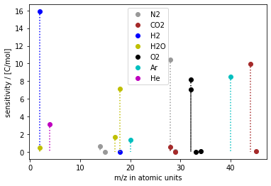
Fig. 7 A calibration, i.e. a set of sensitivity factors, visualized as mass spectrum.
Figure 7 shows a collection of sensitivity factors obtained by calibration.
Predicting sensitivity factors (\(F\)-vs-\(f\))
Sensitivity factors should be measured to the degree possible. If a sensitivity factor cannot be measured, for example due to unavailability in a well-defined and safe form, an approximate predicted value will have to stand in. Here we describe how to predict a sensitivity factor based on the theory presented in Section Step-by-step physics of MS.
If we add the various assumptions and dependencies for all the “internal” transfer functions, represented in Equations (6), (8), (10), (12), and (14) (assuming CEM detector) into Equation (15) defining the sensitivity factor, we get the following expression for \(F\):
(Note that \(M\) here takes on two slightly distinct meanings, first as the mass string defined above in the subscripts, and then as the dimensionless m/z number as the base for the exponents.) The above equation is simplified by joining the constants to \(k_F=k_\mathcal{G}k_\mathcal{I}k_\mathcal{T}k_\mathcal{A}\),and defining \(\beta = \beta_T-\frac{1}{2}\):
For the Faraday cup, we arrive at the same expression just with a different \(k_F\) and \(\beta\).
The least confident assumptions were in the form of the \(M\)-dependency. To acknowledge this, we can replace the simple power-of-\(M\) expression with another form of the “transmission-amplification function” \(\mathcal{T}(M)\).
In general,
However, for now we will assume the \(M^\beta\) dependency and continue from Equation (23).
Finally, to be transparent that this is a predicted and not measured sensitivity factor, and that we know nothing about the constant in front, we rename it from big \(F\) to little \(f\), and replace the supposedly knowable \(k_F\) with an arbitrary constant \(k\) chosen to set
where “M32” should be extended with the setting for which the expression \(f\) will be used.
The equation for \(f\) is then
This little-f sensitivity factor \(f\) serves the purpose of helping to predict big F, the absolute sensitivity factor. They should be directly proportional. The proportionality factor, \(\alpha\), is (due to fact that \(f_\text{M32}^{\text{O}_2}=1\)) equal to the predicted value of the absolute sensitivity of oxygen at m/z=32, \(F_\text{M32}^{\text{O}_2}\), at the setting for which \(f\) will be used.
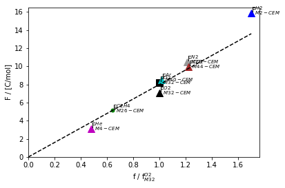
Fig. 8 Measured sensitivity factors vs relative sensitivity factors calculated by Equation (25) for a few common gases at their primary masses with the CEM detector. The fit parameters are \(\alpha=7.98\) [C/mol] and \(\beta=-0.46\). The fit is used here to predict the sensitivity factor for ethylene (C\(_2\)H\(_4\)) at m/z=26 (green dot on the line)
Thus,
or, substituting for \(f\) and assuming the power-of-\(M\) transmission-amplification function motivated above,
\(k\) is defined by Equation (24), so Equation (26) has two free parameters: \(\alpha\) and \(\beta\). These two parameters need to be fit to a set of measured sensitivity factors at a given mass spec setting, and then Equation (26) can be used to predict missing sensitivity factors with the same mass spec setting.
Figure 8 shows an example of this fit. This type of plot is referred to as an “F-vs-f” plot.
- 1
All figures, unless otherwise specified, are made in the accompanying Ipython notebook.